From Point Regression to Roof Slope Detection

Part 2 of 2 in the Roof Face Count series. Previous: Counting Roof Faces: A Dataset of 890K Buildings.

The Modeling Challenge

Given an overhead image of a building, predict the (x, y) location of each roof face. This sounds straightforward, but several properties make it tricky:

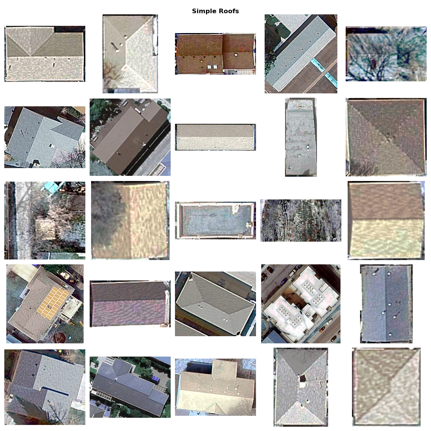
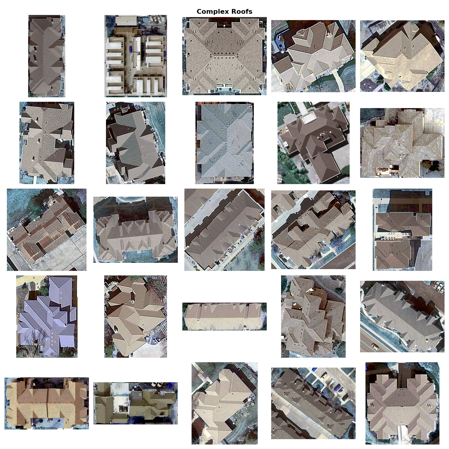
• Variable output size: A simple gable roof has 2 faces; a complex hip-and-valley structure might have 10+. The model must predict a variable number of points.
• Unordered outputs: There’s no natural ordering among roof faces, so the model can’t simply regress a fixed-length vector of coordinates.
• Dense and overlapping: Roof face centers can be close together, especially on complex roofs, making simple heatmap-based approaches prone to merging nearby predictions.

Architecture: Vision Transformer Backbone

After evaluating several backbones, we settled on ViT-L-32 (Vision Transformer, Large, with 32x32 patch size) as the primary feature extractor. The choice was motivated by:

• Global receptive field: Transformers process all patches simultaneously, which is important for reasoning about roof structure—the position of one face constrains where others can be.
• Scale: ViT-L provides sufficient capacity to handle the visual complexity across 835K training images.
• Transfer learning: Pre-trained ViT weights provide strong initialization for overhead imagery.

The model predicts a fixed maximum number of points (up to 11 roof slopes in our experiments) plus an end-of-sequence (EOS) token that signals “no more faces.” During inference, predictions after the EOS token are discarded.

The Loss Function: Hungarian Matching

The unordered nature of the output creates a fundamental challenge: how do you compute loss between a predicted set of points and a ground truth set when you don’t know which prediction should correspond to which target?

We use Hungarian matching (also known as the linear sum assignment problem), the same approach used in DETR for object detection:

1. Compute a cost matrix of distances between all predicted and all ground truth points.
2. Find the optimal one-to-one assignment that minimizes total distance.
3. Compute the loss only on the matched pairs.

This approach is combined with the EOS token loss: the model must learn both where the points are and how many there are.

Loss Components

The final loss combines several terms:

• Matched point distance: Huber loss between each predicted point and its matched ground truth point (more robust to outliers than L2).
• EOS classification loss: Binary cross-entropy for predicting whether each output slot is a real face or past the end of sequence.
• Cosine similarity: An additional geometric constraint encouraging predicted point configurations to match the spatial arrangement of ground truth points.

Training Details

• Dataset: 200K AIRS samples (standardized aerial imagery) for initial training
• Architecture: ViT-L-32 backbone
• Training duration: 500 epochs
• Output: Up to 11 roof slope points per image
• Optimizer: AdamW with cosine learning rate schedule

What Worked and What Didn’t

Iterative Improvements

The path to our best model involved several rounds of ablation:

Gradient issues with cosine similarity loss: Early experiments combining L2 distance with cosine similarity suffered from vanishing gradients. Reducing the learning rate and adding gradient clipping stabilized training.

Sorting predictions before matching: We experimented with pre-sorting predicted points (e.g., left-to-right) before matching, but Hungarian matching without pre-sorting performed better—it allows the model to output points in whatever order is most natural.

Bigger models help: Moving from ResNet-50 to ViT-L-32 provided a significant accuracy boost, justifying the additional compute cost.

SAM-filtered training data matters: Using SAM to isolate single buildings in each training image (rather than feeding in multi-building scenes) substantially improved convergence and final accuracy.

What Underperformed

Heatmap-based counting: GradCAM-based hotspot counting as an auxiliary loss added complexity without consistent improvement—the direct point regression approach was cleaner and more effective.

Contrastive learning with negative samples: Adding images without buildings as negative examples didn’t improve the model, likely because the ViT backbone already handles this well from pre-training.

Dataset Analysis

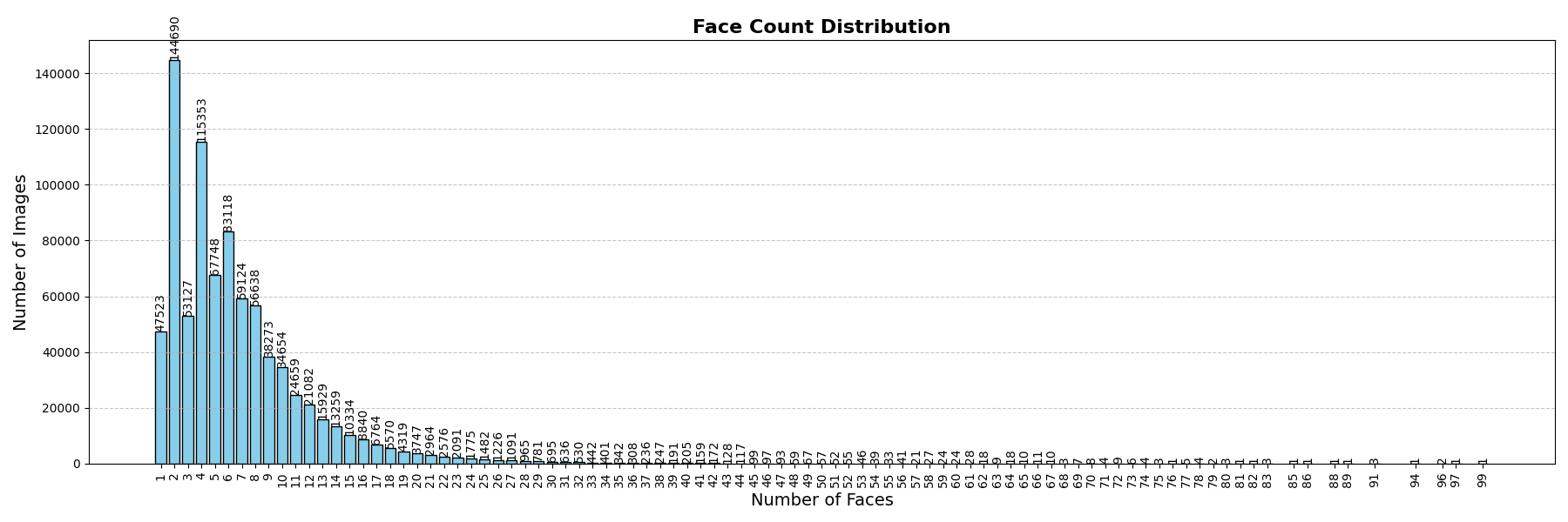
The distribution of roof face counts reveals the challenge: 2-face gable roofs and 4-face hip roofs dominate, but the model must also handle rare complex structures with 8–11+ faces. This long-tailed distribution means the model sees far fewer training examples for complex roofs.

Results and Next Steps

The best model achieves strong accuracy on simple roofs (2–4 faces) and degrades gracefully on complex structures. The ViT-L-32 model trained on 200K AIRS images generalizes surprisingly well to drone imagery, despite the significant domain gap between standardized aerial photos and variable drone captures.

Current directions include:

• Scaling to the full 835K dataset: More diverse training data should improve generalization, especially on complex roofs.
• Ablation studies: Systematically measuring the contribution of each loss component (EOS token, Hungarian matching, cosine similarity).
• From points to edges: Using predicted face centers as seeds for a roof vectorization model that recovers the full wireframe structure.

The ultimate goal is automated roof measurement from a single overhead image—a capability that would transform the roofing, insurance, and solar industries.

Part 2 of 2 in the Roof Face Count series. Previous: Counting Roof Faces: A Dataset of 890K Buildings.